©Richard Lowry, 1999-
All rights reserved.
Chapter 9.
Introduction to Procedures Involving Sample Means
Part 1
In Chapter 5 we introduced the example of a "certain disease that has an abrupt and unmistakable onset, and for which there is currently no effective treatment." In brief, a team of investigators administered a certain plant extract to a certain number of randomly selected patients, beginning for each patient immediately after the onset of the disease and continuing for two months. At the end of a two-month period, they sorted the patients into two outcome categories, "recovered" and "not recovered," and then employed binomial probability procedures to determine whether the number of patients in the "recovered" category was significantly greater than the 40% recovery rate that would have been expected by mere chance coincidence.
It perhaps occurred to you at the time that sorting patients into the two simple categories "recovered" and "not recovered" is rather like a shoe manufacturer producing shoes in only two sizes, "large" and "small." It makes no allowance for the possibility of gradations in-between. Up to a point you could allow for this possibility by sorting the outcomes into a larger number of categories and applying chi-square procedures: for example, "not improved," "somewhat improved," "much improved," and "completely recovered." Even this, however, would potentially leave out much of the fine-grained detail of the reality you are investigating.
Of course there are some distinctions, of the general form "A" and "not-A," that are intrinsically categorical and cannot be measured any other way. For others, such as "conscious,' "semi-conscious," and "unconsciousness," we might have a range of continuous gradations, but with no meaningful way of measuring them. Still, there is a wide range of phenomena for which the finer-grained detail of things can be measured.
Suppose, for example, that a certain normally present component of the patient's blood—component Z—systematically decreases in proportion to the degree of the disease. In this case you could take the concentration of component Z as an inverse measure of the degree of the disease in each particular patient. Providing these measures derived from an equal-interval scale of measurement, you could then also calculate their mean and (pending some other matters yet to be covered) end up being able to say something along the lines of: "On average, patients who received the experimental treatment showed greater improvement than they would have shown if they had not received the treatment." Notice that this is potentially saying quite a lot more than could be said if the outcomes were measured simply as "recovered" and "not recovered." For you can easily imagine a scenario in which patients receiving the experimental treatment show greater improvement, on average, even though the number of full recoveries among them does not exceed the 40% rate to be expected on the basis of mere chance.
The key word in all of this is the phrase "on average." There is a very wide range of research situations where the focus is on the mean of a sample or on the means of two or more samples. This is not simply because science loves averages or the fine-grained measures on an equal-interval scale that averages require. It is because the statistical procedures applicable to this form of measurement are considerably more powerful and versatile. Most of what will be covered in Part 1 of the present chapter is "pure theory," in the sense that it has relatively little immediate practical application. It is, however, very important theory, because it forms the logical groundwork for the eminently useful procedures that we will examine in the chapters following this one. The transition from pure theory to practical application will begin in Part 2 of this chapter; but first we must start at the beginning and build up the logic of it step-by-step.
¶Some Things You Already Know or Could Readily Figure Out
Somewhere deep within the electronic workings of your computer I have created a vast population of Xi values. To prove to you that this population really exists, I have constructed a kind of window through which you can inspect some of its individual constituents. Each time you click the button labeled "N=1," your computer will reach into this population and draw one value of Xi at random. I will ask you to begin by clicking the button twenty or thirty times to gain an intuitive sense of how this population is put together.
The population from which you have just drawn your random values of Xi is shown below in Figure 9.1. As indicated, it is normally distributed with a mean of =18
=18 =±3.
=±3.
Figure 9.1. Reference Source Population, Normally Distributed with=18 and =±3
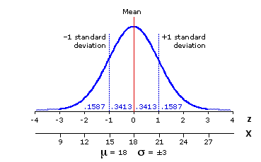
Given that this source population is normally distributed, you know in advance certain facts about how the individual values of Xi sort themselves out. From the proportions listed in the graph (.1587, .3413, etc.), you know at a glance that 34.13% of all instances of Xi fall between the mean and +1 standard deviation; symmetrically, that 34.13% of all instances fall between the mean and —1 standard deviation; and hence, that 68.26% of all values of Xi fall between —1 and +1 standard deviation. Similarly, you know that 15.87% of all instances fall to the left of —1 standard deviation, that an equal 15.87% fall to the right of +1 standard deviation, and so on. Consult the table of the standard normal distribution in Appendix A and you will be able to comb it out in much finer-grained detail. Here again is an abbreviated version of that table, just to remind you of how it is laid out.
Table 9.1. Proportions of the Normal Distribution Falling to the Left of Negative Values of z or to the Right of Positive Values of z.
As we noted in a somewhat different connection in Chapter 6, this detailed knowledge of the properties of a normal distribution puts us in a position to answer all sorts of questions concerning matters of probability. For example: If you were to reach into the source population and select one instance of Xi at random, what is the probability that its value would fall between 18 and 21? ~~ Take another look at Figure 9.1 (shown again below), and the answer practically jumps off the page. Within the source population 34.13% of all instances of Xi fall between the mean (18) and +1 standard deviation (21). Hence:P=.3413.
Similarly for this one: If you were to reach into the source population and select one instance of Xi at random, what is the probability that its value would be equal to or greater than 21? ~~ Within the source population 15.87% of all instances of Xi fall at or beyond +1 standard deviation (21). Hence:P=.1587.
Or for this "two-tailed" variation on the same theme: If you were to reach into the source population and select one instance of Xi at random, what is the probability that its value would be at least 3 points distant from the mean of the population? [That is:Xi < 15 or Xi > 21.] ~~ Within the source population 15.87% of all instances of Xi fall to the left of —1 standard deviation (15), and an equal 15.87% fall to the right of +1 standard deviation (21). Hence: P=.1587+.1587=.3174.
In fact, you could answer any probability question of this general type through the simple strategy of converting the relevant information into units of z, which is to say, into units of standard deviation. The version of z introduced in Chapter 6
pertains only to the special case of binomial probability situations. The basic concept is much more general and can be refitted to apply to a wide range of probability situations that are not binomial in nature. Recall that the essential meaning of z is simply "one standard deviation away from the mean." Thus"+1z" signifies "one standard deviation above the mean"; "—2.5z" says "two and one-half standard deviations below the mean"; and so forth. The general, abstract formulaic structure is simply this:
For the present type of situation where we are randomly drawing one value of Xi from a normally distributed source population, it is the source population itself that constitutes the sampling distribution. Hence the general structure translates into
Thus, a value of Xi=22 drawn from our reference population would be correspond to az-ratio of
For Xi=12 it would be
And so on. From the table of the normal distribution (Appendix A) you will see thatz=+1.33 marks the point beyond which (away from the mean, to the right) fall 9.18% of all possible instances of Xi, while z=—2.0 marks the point beyond which (away from the mean, to the left) fall only a scant 2.28% of all possible instances of Xi. Thus, the probability that a randomly drawn value of Xi will be equal to or greater than 22 is P=.0918, while the probability that it will be equal to or smaller than 12 is .0228.
Everything up to this point should be fairly obvious on the basis of what we covered in Chapter 6. Now we take the same logic a step further.
¶The Sampling Distribution of Sample Means
Among the remarkable properties of a normal distribution is the fact that it is capable of generating other distributions, which are also normal, and which can in turn be used to make probability assessments of a more complex and sophisticated kind. For example, imagine you were to draw a vast number of random samples from our source population, each sample ofsize N=10. If you were then to take the means of all those samples and lay them out in the form of a frequency distribution, the result would be a very close approximation of the theoretical sampling distribution shown in Figure 9.2. As this is a distribution composed of sample means (M), we label its mean as M and its standard deviation as M.
Figure 9.2. Sampling Distribution of the Means of Samples of Size N=10 Randomly Drawn from a Normally Distributed Source Population with=18 and =±3
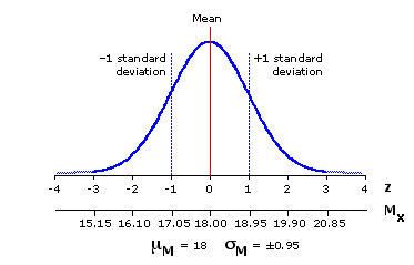
The fact that this sampling distribution of sample means is normally distributed is only the first part of the story. Equally important is that the two main parameters of the sampling distribution, its central tendency and variability, will be systematically related to those of the source population. Indeed, the means of the two distributions will be identical. As illustrated by the present example, the mean of the source population is 18.0, and so too is the mean of the sampling distribution of means. For this or any other situation where samples of size N are randomly drawn from a normally distributed source population, the relationship is
The reason for this identity is simply that both distributions are constructed of the same basic elements. In drawing random samples of size N from the source population, all we are really doing is randomly sorting the individual values of Xi from the source population into numerous groups, each of size N. The overall mean of all these items will be the same no matter how we sort them.
The respective variabilities of the two distributions are also precisely related, although here the relationship is somewhat more complex since it must take into account not only the variability of the source population but also the size of the samples that are being drawn from it. The basic logic of this point is that the properties of the source population will tend to be more accurately reflected by a larger sample than by a smaller one. In particular, the larger the sample, the greater the likelihood that its mean will approximate the mean of the population from which it is drawn. The result is that the means of larger samples will tend to cluster more tightly around the mean of the source population, while those of smaller samples will cluster more loosely and disperse more widely.
To illustrate this point more concretely, suppose we were drawing samples of different sizes from our reference source population. For samples of relatively small size, a single extreme Xi value such as 13 or 24 would have a relatively large effect on the mean of the sample. With samples of size N=2, for instance, we could quite easily get two sample values such as 18 and 24, which would yield a sample mean of 21; or such as 18 and 12, which would produce a sample mean of 15. With samples of larger size, however, occasional extreme values such as 12 and 24 will have a proportionately smaller effect upon sample means because they are now being averaged in with a larger number of more moderate values such as 17, 18, and 19.
The precise form of the relationship can be expressed in terms of either variance (2) or standard deviation (). When drawing random samples of size N from a normally distributed source population:
Thus for samples of size N=4 drawn from our reference source population, the standard deviation of the sampling distribution of means would be
For samples of size N=10 it would be
And so forth. In each of these two cases, 68.26% of all sample means would fall within the range bounded by —1 and +1 standard deviation, that is, between—1M and +1M. However, for the N=4 sampling distribution this interval is relatively wide (±1.5), whereas for the N=10 sampling distribution it is relatively narrow (±0.95). In the N=4 distribution you would find 68.26% of all sample means falling between 16.5 and 19.5, while in the N=10 distribution you would find the same proportion clustering more compactly between 17.05 and 18.95. For samples of size N=20 (M=±0.67) the middle 68.26% of the sampling distribution would cluster even more compactly between 17.33 and 18.67; for samples of size N=40 (M=±0.47), still more compactly between 17.53 and 18.47; and so on.
The upshot of all this is that if you know a source population to be normally distributed, and if you happen also to know the values of its mean and standard deviation, you are then in a position to answer all sorts of probability questions concerning the means of such samples as might be drawn from that source population. For example: If you were to draw from our reference source population one random sample of size N=10, what is the probability that the mean of the sample would be equal to or greater than 20? Here again is Figure 9.2, which shows the sampling distribution that would apply to this scenario.
Figure 9.2 [Repeated]. Sampling Distribution of the Means of Samples of Size N=10 Randomly Drawn from a Normally Distributed Source Population with=18 and =±3
It will be obvious at a glance that a sample mean as large as MX=20 would be fairly unlikely to occur through mere chance coincidence, falling as it does at about two standard deviations away from the mean of the sampling distribution. We saw earlier in this chapter that the general structure of a z-ratio
can be tailored to apply to a variety of situations. In the present case, the tailoring takes the form
From the table of the normal distribution (Appendix A) you will see thatz=+2.11 marks the point beyond which (away from the mean, to the right) fall 1.74% of all the possible sample means that might result from a random sample of size N=10. Thus, the probability that the mean of any particular sample of size N=10 will be equal to or greater than 20 is a scant 0.0174. Falling at the same distance at the opposite extreme of the sampling distribution (z=—2.11), hence equally unlikely, would be a sample mean equal to or smaller than 16. The probability of ending up with a sample mean as small as 16 (MX < 16) or as large as 20 (MX > 20) is therefore 0.0174+0.0174=0.0348.
Here again is an opportunity to click a button. Each time you click the one below, labeled "N=10," your computer will reach into the reference source population and draw a sample of 10 random values of Xi. It will also calculate and display the means(MX) of your samples, both separately and cumulatively. Please click the button twenty or thirty times, taking particular note of the following as your sample means accumulate:
¶The Sampling Distribution of Sample-Mean Differences
Now for a somewhat more complex variation on the same theme. Suppose we were to reach into our reference source population and draw a vast number of pairs of samples. We will designate the first sample in each pair as A, the second as B, and stipulate that their respective sizes are Na and Nb. For each pair we take the difference between the mean of sample A and the mean of sample B, according to the formula
difference = MXa—MXb
and then at the end we sort out all of these sample-mean differences in the form of a frequency distribution.
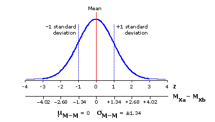
Here as well we would end up with a sampling distribution that is normal in form and whose properties would be systematically related to those of the source population from which the samples are drawn. The average of all sample means of type-A would be equal to the mean of the source population(source=18), and so too would be the average of all sample means of type-B. The average difference between type-A and type-B sample means would therefore be zero, and the mean of this sampling distribution of sample-mean differences (subscripted as "M-M") would accordingly be
M-M = 0
The measures of variability for this sampling distribution are determined on the one hand by the amount of variability that exists within the source population and on the other by the sizes of the two types of samples, Na and Nb. When drawing pairs of random samples of sizes Na and Nb from a normally distributed source population:
Although we have not yet explicitly specified the variance of our source population, you will know that it must be2source=9, since its standard deviation, which is simply the square root of the variance, is source=±3. Thus for the case where we are drawing random samples of sizes Na=10 and Nb=10 from our source population, the standard deviation of the relevant sampling distribution would be
Figure 9.3 shows the outlines of the sampling distribution of sample-mean differences for the case where the source population is normally distributed with a mean of 18 and a standard deviation of ±3, and where the samples oftype-A and type-B are of sizes Na=10 and Nb=10. The same general outlines would appear for any other values of Na and Nb. The only difference would be in the value of M-M, the standard deviation of the sampling distribution.
Figure 9.3. Sampling Distribution of Sample-Mean Differences, for Samples of SizesNa=10 and Nb=10 Randomly Drawn from a Normally Distributed Source Population with =18 and =±3
You will certainly be able to guess where we go next. Suppose you were to reach into our reference source population and draw two random samples, A and B, each of size N=10. Three questions:
To answer questions of this type, we once again take the general structure of az-ratio
and refit it to apply to the current situation. Now the re-tailoring takes the form
As indicated above, the mean of the sampling distribution will always beM-M=0 (except for certain specialized applications that we need not go into just now). So it can simply be dropped out of the equation to yield
Thus for Question 1, the probability that [MXa—MXb] > 2:
And for Question 2, the probability that [MXa—MXb] < —2:
From the table of the normal distribution (Appendix A) you will see thatz=+1.49 marks the point beyond which (away from the mean, to the right) fall 6.81% of all the possible differences between MXa and MXb in this particular scenario. The probability (Question 1) that the mean of sample A will be 2 or more points greater than the mean of sample B in any randomly drawn pair of samples is therefore 0.0681. The same is true of z=—1.49, though in the opposite direction. So 0.0681 is also the probability (Question 2) that the mean of sample B will be 2 or more points greater than the mean of sample A in any randomly drawn pair of samples. The sum of these two will give the disjunctive probability (Question 3) of finding at least a 2-point difference between the means of sample A and sample B, in either direction: 0.0681+0.0681=0.1362.
One more button-click exercise, and then we will move on to see how all this abstract theory can be adapted to purposes of practical application. Below is a button labeled "Two Samples." Each time you click it, your computer will draw two random samples from our normally distributed reference population, each of size N=10. If you have the patience to click the button several hundred times, you will find the proportions of the types of outcomes stipulated in Questions 1, 2, and 3 approaching closer and closer to the theoretical proportions of 0.0681, 0.0681, and 0.1362.
Vocabulary Note:
End of Chapter 9, Part 1.It perhaps occurred to you at the time that sorting patients into the two simple categories "recovered" and "not recovered" is rather like a shoe manufacturer producing shoes in only two sizes, "large" and "small." It makes no allowance for the possibility of gradations in-between. Up to a point you could allow for this possibility by sorting the outcomes into a larger number of categories and applying chi-square procedures: for example, "not improved," "somewhat improved," "much improved," and "completely recovered." Even this, however, would potentially leave out much of the fine-grained detail of the reality you are investigating.
Of course there are some distinctions, of the general form "A" and "not-A," that are intrinsically categorical and cannot be measured any other way. For others, such as "conscious,' "semi-conscious," and "unconsciousness," we might have a range of continuous gradations, but with no meaningful way of measuring them. Still, there is a wide range of phenomena for which the finer-grained detail of things can be measured.
Suppose, for example, that a certain normally present component of the patient's blood—component Z—systematically decreases in proportion to the degree of the disease. In this case you could take the concentration of component Z as an inverse measure of the degree of the disease in each particular patient. Providing these measures derived from an equal-interval scale of measurement, you could then also calculate their mean and (pending some other matters yet to be covered) end up being able to say something along the lines of: "On average, patients who received the experimental treatment showed greater improvement than they would have shown if they had not received the treatment." Notice that this is potentially saying quite a lot more than could be said if the outcomes were measured simply as "recovered" and "not recovered." For you can easily imagine a scenario in which patients receiving the experimental treatment show greater improvement, on average, even though the number of full recoveries among them does not exceed the 40% rate to be expected on the basis of mere chance.
The key word in all of this is the phrase "on average." There is a very wide range of research situations where the focus is on the mean of a sample or on the means of two or more samples. This is not simply because science loves averages or the fine-grained measures on an equal-interval scale that averages require. It is because the statistical procedures applicable to this form of measurement are considerably more powerful and versatile. Most of what will be covered in Part 1 of the present chapter is "pure theory," in the sense that it has relatively little immediate practical application. It is, however, very important theory, because it forms the logical groundwork for the eminently useful procedures that we will examine in the chapters following this one. The transition from pure theory to practical application will begin in Part 2 of this chapter; but first we must start at the beginning and build up the logic of it step-by-step.
¶Some Things You Already Know or Could Readily Figure Out
Somewhere deep within the electronic workings of your computer I have created a vast population of Xi values. To prove to you that this population really exists, I have constructed a kind of window through which you can inspect some of its individual constituents. Each time you click the button labeled "N=1," your computer will reach into this population and draw one value of Xi at random. I will ask you to begin by clicking the button twenty or thirty times to gain an intuitive sense of how this population is put together.
Xi = |
The population from which you have just drawn your random values of Xi is shown below in Figure 9.1. As indicated, it is normally distributed with a mean of
Figure 9.1. Reference Source Population, Normally Distributed with
Given that this source population is normally distributed, you know in advance certain facts about how the individual values of Xi sort themselves out. From the proportions listed in the graph (.1587, .3413, etc.), you know at a glance that 34.13% of all instances of Xi fall between the mean and +1 standard deviation; symmetrically, that 34.13% of all instances fall between the mean and —1 standard deviation; and hence, that 68.26% of all values of Xi fall between —1 and +1 standard deviation. Similarly, you know that 15.87% of all instances fall to the left of —1 standard deviation, that an equal 15.87% fall to the right of +1 standard deviation, and so on. Consult the table of the standard normal distribution in Appendix A and you will be able to comb it out in much finer-grained detail. Here again is an abbreviated version of that table, just to remind you of how it is laid out.
Table 9.1. Proportions of the Normal Distribution Falling to the Left of Negative Values of z or to the Right of Positive Values of z.
| ±z 0.00 0.20 0.40 0.60 0.80 1.00 1.20 1.40 1.60 | Area Beyond ±z .5000 .4207 .3446 .2743 .2119 .1587 .1151 .0808 .0548 | ±z 1.80 2.00 2.20 2.40 2.60 2.80 3.00 3.50 4.00 | Area Beyond ±z .0359 .0228 .0139 .0082 .0047 .0026 .0013 .0002 .00003
| | |||||||
As we noted in a somewhat different connection in Chapter 6, this detailed knowledge of the properties of a normal distribution puts us in a position to answer all sorts of questions concerning matters of probability. For example: If you were to reach into the source population and select one instance of Xi at random, what is the probability that its value would fall between 18 and 21? ~~ Take another look at Figure 9.1 (shown again below), and the answer practically jumps off the page. Within the source population 34.13% of all instances of Xi fall between the mean (18) and +1 standard deviation (21). Hence:
Similarly for this one: If you were to reach into the source population and select one instance of Xi at random, what is the probability that its value would be equal to or greater than 21? ~~ Within the source population 15.87% of all instances of Xi fall at or beyond +1 standard deviation (21). Hence:
Or for this "two-tailed" variation on the same theme: If you were to reach into the source population and select one instance of Xi at random, what is the probability that its value would be at least 3 points distant from the mean of the population? [That is:
In fact, you could answer any probability question of this general type through the simple strategy of converting the relevant information into units of z, which is to say, into units of standard deviation. The version of z introduced in Chapter 6
| z = | (k— | | k = the observed value binomial sampling distribution binomial sampling distribution |
pertains only to the special case of binomial probability situations. The basic concept is much more general and can be refitted to apply to a wide range of probability situations that are not binomial in nature. Recall that the essential meaning of z is simply "one standard deviation away from the mean." Thus
| z = | (observed value)—(mean of the relevant sampling distribution) standard deviation of the relevant sampling distribution |
For the present type of situation where we are randomly drawing one value of Xi from a normally distributed source population, it is the source population itself that constitutes the sampling distribution. Hence the general structure translates into
| z = | Xi— | | Xi = the observed or stipulated value Note that there is no "±.5" correction for continuity in this formulation.
| | |||||
Thus, a value of Xi=22 drawn from our reference population would be correspond to a
| z = | 22—18 3 | = +1.33··· |
For Xi=12 it would be
| z = | 12—18 3 | = —2.0 |
And so on. From the table of the normal distribution (Appendix A) you will see that
Everything up to this point should be fairly obvious on the basis of what we covered in Chapter 6. Now we take the same logic a step further.
¶The Sampling Distribution of Sample Means
Among the remarkable properties of a normal distribution is the fact that it is capable of generating other distributions, which are also normal, and which can in turn be used to make probability assessments of a more complex and sophisticated kind. For example, imagine you were to draw a vast number of random samples from our source population, each sample of
Figure 9.2. Sampling Distribution of the Means of Samples of Size N=10 Randomly Drawn from a Normally Distributed Source Population with
The fact that this sampling distribution of sample means is normally distributed is only the first part of the story. Equally important is that the two main parameters of the sampling distribution, its central tendency and variability, will be systematically related to those of the source population. Indeed, the means of the two distributions will be identical. As illustrated by the present example, the mean of the source population is 18.0, and so too is the mean of the sampling distribution of means. For this or any other situation where samples of size N are randomly drawn from a normally distributed source population, the relationship is
of sample means |
The reason for this identity is simply that both distributions are constructed of the same basic elements. In drawing random samples of size N from the source population, all we are really doing is randomly sorting the individual values of Xi from the source population into numerous groups, each of size N. The overall mean of all these items will be the same no matter how we sort them.
The respective variabilities of the two distributions are also precisely related, although here the relationship is somewhat more complex since it must take into account not only the variability of the source population but also the size of the samples that are being drawn from it. The basic logic of this point is that the properties of the source population will tend to be more accurately reflected by a larger sample than by a smaller one. In particular, the larger the sample, the greater the likelihood that its mean will approximate the mean of the population from which it is drawn. The result is that the means of larger samples will tend to cluster more tightly around the mean of the source population, while those of smaller samples will cluster more loosely and disperse more widely.
To illustrate this point more concretely, suppose we were drawing samples of different sizes from our reference source population. For samples of relatively small size, a single extreme Xi value such as 13 or 24 would have a relatively large effect on the mean of the sample. With samples of size N=2, for instance, we could quite easily get two sample values such as 18 and 24, which would yield a sample mean of 21; or such as 18 and 12, which would produce a sample mean of 15. With samples of larger size, however, occasional extreme values such as 12 and 24 will have a proportionately smaller effect upon sample means because they are now being averaged in with a larger number of more moderate values such as 17, 18, and 19.
The precise form of the relationship can be expressed in terms of either variance (
| the variance of the sampling distribution of sample means is equal to the variance of the source population divided by N |
| x | x N | x x |
| and the standard deviation of the sampling distribution of sample means is equal to the standard deviation of the source population divided by the square root of N |
| x | x sqrt[N] | x x |
Thus for samples of size N=4 drawn from our reference source population, the standard deviation of the sampling distribution of means would be
| x | ±3 sqrt[4] | = ±1.5 |
For samples of size N=10 it would be
| x | ±3 sqrt[10] | = ±0.95 |
And so forth. In each of these two cases, 68.26% of all sample means would fall within the range bounded by —1 and +1 standard deviation, that is, between
The upshot of all this is that if you know a source population to be normally distributed, and if you happen also to know the values of its mean and standard deviation, you are then in a position to answer all sorts of probability questions concerning the means of such samples as might be drawn from that source population. For example: If you were to draw from our reference source population one random sample of size N=10, what is the probability that the mean of the sample would be equal to or greater than 20? Here again is Figure 9.2, which shows the sampling distribution that would apply to this scenario.
Figure 9.2 [Repeated]. Sampling Distribution of the Means of Samples of Size N=10 Randomly Drawn from a Normally Distributed Source Population with
It will be obvious at a glance that a sample mean as large as MX=20 would be fairly unlikely to occur through mere chance coincidence, falling as it does at about two standard deviations away from the mean of the sampling distribution. We saw earlier in this chapter that the general structure of a z-ratio
| z = | (observed value)—(mean of the relevant sampling distribution) standard deviation of the relevant sampling distribution |
can be tailored to apply to a variety of situations. In the present case, the tailoring takes the form
| z = | MX— | = | 20—18 0.95 | = +2.11 |
MX = observed sample mean |
From the table of the normal distribution (Appendix A) you will see that
Here again is an opportunity to click a button. Each time you click the one below, labeled "N=10," your computer will reach into the reference source population and draw a sample of 10 random values of Xi. It will also calculate and display the means
Within each sample, occasional extreme values of Xi will tend to be balanced off by the other values of Xi in the sample. In consequence, the means of the samples will tend to fall fairly close to the sampling distribution mean of Few if any of your sample means will be as small as 16 or as large as 20. If you were to continue clicking the "N=10" button several hundred times, you would find the proportions of such extreme sample means coming closer and closer to the theoretical proportions of 0.0174 |
| Xi | Sample Means|
|
|
|
| | |||
¶The Sampling Distribution of Sample-Mean Differences
Now for a somewhat more complex variation on the same theme. Suppose we were to reach into our reference source population and draw a vast number of pairs of samples. We will designate the first sample in each pair as A, the second as B, and stipulate that their respective sizes are Na and Nb. For each pair we take the difference between the mean of sample A and the mean of sample B, according to the formula
and then at the end we sort out all of these sample-mean differences in the form of a frequency distribution.
Here as well we would end up with a sampling distribution that is normal in form and whose properties would be systematically related to those of the source population from which the samples are drawn. The average of all sample means of type-A would be equal to the mean of the source population
The measures of variability for this sampling distribution are determined on the one hand by the amount of variability that exists within the source population and on the other by the sizes of the two types of samples, Na and Nb. When drawing pairs of random samples of sizes Na and Nb from a normally distributed source population:
| the variance of the sampling distribution of sample-mean differences (again subscripted as plusa the variance of the source population divided by Nb |
| x | x Na | + | x Nb | x x |
| and the standard deviation of the sampling distribution of sample-mean differences is equal to the square root of this quantity |
| x | [ | x Na | + | x Nb | ] |
Although we have not yet explicitly specified the variance of our source population, you will know that it must be
| x | [ | 9 10 | + | 9 10 | ] | = ±1.34 |
Figure 9.3 shows the outlines of the sampling distribution of sample-mean differences for the case where the source population is normally distributed with a mean of 18 and a standard deviation of ±3, and where the samples of
Figure 9.3. Sampling Distribution of Sample-Mean Differences, for Samples of Sizes
You will certainly be able to guess where we go next. Suppose you were to reach into our reference source population and draw two random samples, A and B, each of size N=10. Three questions:
| Question 1 | Question 2 | Question 3| What is the probability that the mean of sample A will be 2 or more points greater than the mean of sample B? | [MXa—MXb] > 2 What is the probability that the mean of sample B will be 2 or more points greater than the mean of sample A? | [MXa—MXb] < —2 What is the probability that there will be at least a 2-point difference between the means of the two samples, in either direction? | [MXa—MXb] > 2 or [MXa—MXb] < —2 |
To answer questions of this type, we once again take the general structure of a
| z = | (observed value)—(mean of the relevant sampling distribution) standard deviation of the relevant sampling distribution |
and refit it to apply to the current situation. Now the re-tailoring takes the form
| z = | [MXa—MXb] —
| MXa = mean of sample A MXb = mean of sample B |
As indicated above, the mean of the sampling distribution will always be
| z = | MXa—MXb |
Thus for Question 1, the probability
| z = | MXa—MXb | = | 2 1.34 | = +1.49 |
And for Question 2, the probability that [MXa—MXb] < —2:
| z = | MXa—MXb | = | —2 1.34 | = —1.49 |
From the table of the normal distribution (Appendix A) you will see that
One more button-click exercise, and then we will move on to see how all this abstract theory can be adapted to purposes of practical application. Below is a button labeled "Two Samples." Each time you click it, your computer will draw two random samples from our normally distributed reference population, each of size N=10. If you have the patience to click the button several hundred times, you will find the proportions of the types of outcomes stipulated in Questions 1, 2, and 3 approaching closer and closer to the theoretical proportions of 0.0681, 0.0681, and 0.1362.
Vocabulary Note:
|
"standard deviation of the sampling distribution of sample means" | You will often find this quantity spoken of as the "standard error of the mean."
|
"standard deviation of | the sampling distribution of sample-mean differences" By extension, you could speak of this quantity as the "standard error of sample-mean differences." In general, the "standard error" of a statistic (sample means, sample-mean differences, etc.) is the standard deviation of the sampling distribution of that statistic.
| |
Return to Top of Chapter 9, Part 1
Go to Chapter 9, Part 2
| Home | Click this link only if the present page does not appear in a frameset headed by the logo Concepts and Applications of Inferential Statistics |