©Richard Lowry, 1999-
All rights reserved.
Chapter 7.
Tests of Statistical Significance: Three Overarching Concepts
Although sampling distributions often have an intellectual elegance and beauty in and of themselves, their chief function lies in the workaday realm of practical application. They are the devices by which scientific researchers can rationally determine how confident they may be that their observed results reflect anything more than mere chance coincidence. In Chapter 6 we introduced the general concept of sampling distributions via the particular example of binomial distributions, along with the normal distribution whose form and properties the binomial distributions tend to approximate. Before going on to consider other sampling distributions and their associated tests of statistical significance, we will take a moment to draw out some further details concerning the general concept of statistical significance.
¶Mean Chance Expectation
All tests of statistical significance involve a comparison between
A useful generic label for the second of these values is mean chance expectation, which we can abbreviate as MCE. For binomial probability situations of the sort described in Chapter 6, MCE is in every case equal to the mean, , of the relevant binomial sampling distribution. Thus, for the case of 10 coin tosses, MCE for the number of heads is
If you actually perform 10 coin tosses, it is of course entirely possible that you might end up with as many as 6 or 7 or 8 heads, or as few as 4 or 3 or 2. Indeed, there is a 1/1,024 chance—small, but nonetheless greater than zero—of ending up with all 10 heads, and an equal 1/1,024 chance of ending up with no heads at all. When we say that MCE for heads in this situation is 5, the reference is not to 5 exactly but to 5 probabilistically. Essentially, it is the concept of a sampling distribution expressed in somewhat different language. Within the entire range of possible outcomes in this situation—zero heads, 1 head, 2 heads, and so on, up through 10 heads—the closer a particular outcome is to the MCE value of 5, the more likely it is to occur by mere chance coincidence; and conversely, the farther away it falls from the MCE value of 5, the less likely it is to occur by mere chance coincidence. To help consolidate your grasp of this concept, the following graph shows the outlines of the binomial sampling distribution for this situation, and the table beneath it lists the respective probabilities for each of the 11 possible outcomes.
¶The Null Hypothesis and the Research Hypothesis
~~~~
In this section and the one that follows, we will be taking some familiar items of symbolic notation—"=," "not=," ">," and "<"—and printing them in blue to convey the concepts of random variability and statistical significance. When you encounter these blue symbols, they are to be read as follows:
~~~~
When performing a test of of statistical significance, it is a useful convention to distinguish between
The second of these items is commonly spoken of as the null hypothesis, the word "null" in this context having essentially the meaning of "zero." Hence its conventional symbolic notation, H0, which is H for "hypothesis," with a subscripted zero. The research hypothesis, on the other hand, sometimes also spoken of as the experimental hypothesis or alternative hypothesis, is typically symbolized as H1. In general, the null hypothesis is to the effect that the observed result—e.g., the number of patient recoveries—will not significantly differ from mean chance expectation; in other words, that it will be equal to MCE, within the limits of random variability:
H0: observed value = MCE
And the research hypothesis is to the effect that there will be a significant difference between the observed result and MCE.
H1: observed value not= MCE [tentative!]
The specific form of the research hypothesis can be either directional or non-directional, depending upon the particular question that is at issue in the research. The version of H1 that we have just given is non-directional, in that it asserts there will be a difference between the observed result and MCE, but makes no claim about the particular direction of the difference. It is tantamount to saying: There will be a significant difference between the observed result and MCE, though we have no basis for predicting in just which direction the difference will go, and will therefore take a significant difference in either direction as support for our hypothesis. A directional hypothesis, on the other hand, is one that does specify the particular direction of the difference. In the medication experiment described in Chapter 6, for example, the investigators did not merely hypothesize that the observed number of patient recoveries would be different from MCE; their specific hypothesis was that it would be greater than MCE:
H1: observed value > MCE [directional H1]
Had they instead been examining the effect of sleep deprivation on the outcome of the disease, they might have had reason to expect that the number of recoveries would be smaller than MCE.
H1: observed value < MCE [directional H1]
As we noted when first mentioning this matter in Chapter 4, a non-directional hypothesis is essentially an either-or combination of the two forms of directional hypotheses. Thus, when we put forward a non-directional hypothesis of the general type
H1: observed value not= MCE [non-directional H1]
what we are really saying is
Although this form of research hypothesis is conventionally spoken of as non-directional, you will see from this breakdown of it that the more accurate label would be bi-directional.
¶Directional versus Non-directional Research Hypotheses and One-Way versus Two-Way Tests of Significance
The distinction between a directional and a non-directional hypothesis is not just a matter of using the right words in the right place. It also marks a very important distinction in logic. To illustrate the nature of this distinction, return for a moment to that fanciful mind-over-matter coin-toss example introduced at the beginning of Chapter 5; except now we will examine it in two different versions.
Scenario 1. As we described it at the time, our claimant of paranormal powers was aiming to produce "an impressive number of heads, to the point where you will at least be willing to take my claim seriously." Putting him to the test, we toss the coin 100 times and find that 59 of these tosses come up as heads. As the observed number of heads is only 9 greater than the 50 that we would calculate as MCE, you are perhaps not very impressed by this result at first glance. Upon closer examination, however, you find that this particular binomial outcome (with N=100, k=59, p=.5 and q=.5) yields a z-ratio of +1.7 which, as shown in Figure 7.1, is associated with a probability of only P=.0446.
Figure 7.1 Location of z=+1.7 in the Unit Normal Distribution
That is: Of all the combinations of heads and tails that might occur by mere chance in 100 tosses of a coin, only 4.46% of them would include as many as 59 heads. So the result in this scenario is significant a bit beyond the conventional .05 level.
Scenario 2. Suppose that our mind-over-matter claimant had instead asserted the following:
Putting him to the test, we toss the coin 100 times and find that 59 of these tosses come up as heads.
Although both of these scenarios have a total of 100 tosses and end up with 59 heads instead of the 50 of MCE, the logic of probability in the two cases is quite different. In Scenario 1 the research hypothesis is directional, explicitly stating at the outset that the observed number of heads will be greater than the MCE value of 50:
H1: observed no. of heads > MCE
while in Scenario 2 it is non-directional, which is to say, bi-directional.
So when you assess statistical significance in these two scenarios, you are really asking two quite different questions. In Scenario 1 the question takes the specific directional form
whereas in Scenario 2 it takes the form
And clearly, the mere-chance probability for "either heads or tails" is greater than for just "heads." Figure 7.2 is the same as Figure 7.1, except now we show the probabilities for both sides of the either/or outcome. The probability of ending up with as many as 59 heads is P=.0446, whereas the probability for ending up with as many as 59 heads or as many as 59 tails is twice that amount, P=.0892.
Figure 7.2 Locations of z=±1.7 and in the Unit Normal Distribution
Thus, by the conventional standard of statistical significance (P<.05), the observed result in Scenario 1 is significant (P=.0446), while the one in Scenario 2 is not (P=.0892). As you first encounter this logical distinction between directional and non-directional hypotheses, you are likely to find it a bit bizarre; for, after all, the observed fact is what it is, irrespective of whatever expectations we might have had about it prior to its occurrence. The 100 tosses and 59 heads that occur in Scenarios 1 and 2, respectively, do not materially differ from one another in any discernible way. So why should the probability of one 59-heads outcome be .0446 and the probability of the other be .0892? The answer is actually a rather simple one, though it will need to move around in your mind a bit before it comfortably settles down. It is simply that, when we perform a test of statistical significance, what we are testing is not the observed fact in and of itself, but rather the hypothesis to which the fact is connected. In general, the assessment of probability in connection with a directional hypothesis is spoken of as a one-way test, while the assessment for a non-directional (i.e., bi-directional) hypothesis is called a two-way test. Because such tests often refer to the left- and right-side "tails" of a symmetrical sampling distribution (as in Figure 7.2), they are also often described as one-tail and two-tail tests. As a practical rule of thumb, the probability of any particular observed result assessed by a two-way test is either exactly or approximately twice the probability that would be assessed for a one-way test.
The logic of the non-directional hypothesis is also the default position when there is no prior hypothesis at all. For example, imagine that you cut class on the day that the experiments of Scenarios 1 and 2 take place and thus know nothing about them. To amuse yourself, as well as to take the edge off the shame you rightly feel for cutting class, you toss a coin 16 times to see how closely the outcomes approximate the 8 heads and 8 tails that you now know would be calculated as MCE. Counting up a total of 12 heads among the observed outcomes, and only 4 tails, you excitedly say to yourself: "Hey, look at all those heads! P=.04. I must have the power of mind over matter!"
Figure 7.3 Binomial Sampling Distribution for p=.5, q=.5, and N=16
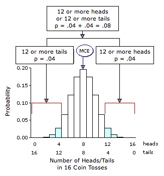
But the fact is that you were not expecting or aiming for heads. Essentially, you were saying "Let's do this and see what happens"; and your hypothesis, at most, was that the obtained result might prove different from MCE, in one direction or the other. The proof of this logical pudding is that, if the outcome were 12 tails instead of 12 heads, your reaction would be exactly the same, except now it would be occasioned by the obverse side of the coin: "Hey, look at all those tails! P=.04. I must have the power of mind over matter!" Given the bi-directional nature of your implicit hypothesis, the probability that would be assessed for either of these outcomes would notbe .04, but rather .04+.04=.08.
We now move on to consider some tests of statistical significance that can be performed using a highly versatile family of procedures collectively known as chi-square.
¶Mean Chance Expectation
All tests of statistical significance involve a comparison between
(i) an observed value and |
E.g., an observed correlation coefficient; an observed number of heads in N tosses of a coin; an observed number of recoveries in N patients; and so on.
| (ii) the value that one would expect to find, on average, if nothing other than chance coincidence, mere random variability, were operating in the situation.
|
| E.g., a correlation coefficient of r=0, assuming that the correlation within the general population of paired XiYi values is rho=0; 5 heads in 10 tosses of a coin, assuming that the mere chance probability of a head on any particular toss is p=.5; 400 recoveries in 1,000 patients, assuming that the probability of mere chance recovery for any particular patient is p=.4; and so on. |
A useful generic label for the second of these values is mean chance expectation, which we can abbreviate as MCE. For binomial probability situations of the sort described in Chapter 6, MCE is in every case equal to the mean,
| MCE(heads) | = |
Where N=10, the number of tosses, and p=.5, the probability of a head on any particular one of the N tosses.
|
| = 10 x .5 = 5 | |
If you actually perform 10 coin tosses, it is of course entirely possible that you might end up with as many as 6 or 7 or 8 heads, or as few as 4 or 3 or 2. Indeed, there is a 1/1,024 chance—small, but nonetheless greater than zero—of ending up with all 10 heads, and an equal 1/1,024 chance of ending up with no heads at all. When we say that MCE for heads in this situation is 5, the reference is not to 5 exactly but to 5 probabilistically. Essentially, it is the concept of a sampling distribution expressed in somewhat different language. Within the entire range of possible outcomes in this situation—zero heads, 1 head, 2 heads, and so on, up through 10 heads—the closer a particular outcome is to the MCE value of 5, the more likely it is to occur by mere chance coincidence; and conversely, the farther away it falls from the MCE value of 5, the less likely it is to occur by mere chance coincidence. To help consolidate your grasp of this concept, the following graph shows the outlines of the binomial sampling distribution for this situation, and the table beneath it lists the respective probabilities for each of the 11 possible outcomes.
| 0 | 1 | 2 | 3 | 4 | 5 | 6 | 7 | 8 | 9 | 10
| Number of Heads in 10 Tosses of a Coin
| | |||||||||||||||||||||
| Number of Heads 0 1 2 3 4 5 6 7 8 9 10 | Probability .00098 .00977 .04395 .11719 .20508 .24609 .20508 .11719 .04395 .00977 .00098 |
¶The Null Hypothesis and the Research Hypothesis
~~~~
In this section and the one that follows, we will be taking some familiar items of symbolic notation—"=," "not=," ">," and "<"—and printing them in blue to convey the concepts of random variability and statistical significance. When you encounter these blue symbols, they are to be read as follows:
| a = b | a and b will not significantly differ; that is, a will be equal to b, within the limits of random variability;
| a not= b
|
a and b will significantly differ (there will be a difference between a and b that goes beyond what could be expected on the basis of mere random variability);
| a > b
|
a will be significantly greater than b (a will be greater than b in a degree that goes beyond what could be expected on the basis of mere random variability); and
| a < b
|
a will be significantly smaller than b (a will be smaller than b in a degree that goes beyond what could be expected on the basis of mere random variability).
| |
When performing a test of of statistical significance, it is a useful convention to distinguish between
| (i) | the particular hypothesis that the research is seeking to examine; e.g., that the experimental medication has some degree of effectiveness as a treatment of the disease;
|
| and
|
| (ii)
| the logical antithesis of the research hypothesis; e.g., that the experimental medication has no effectiveness at all.
| |
The second of these items is commonly spoken of as the null hypothesis, the word "null" in this context having essentially the meaning of "zero." Hence its conventional symbolic notation, H0, which is H for "hypothesis," with a subscripted zero. The research hypothesis, on the other hand, sometimes also spoken of as the experimental hypothesis or alternative hypothesis, is typically symbolized as H1. In general, the null hypothesis is to the effect that the observed result—e.g., the number of patient recoveries—will not significantly differ from mean chance expectation; in other words, that it will be equal to MCE, within the limits of random variability:
And the research hypothesis is to the effect that there will be a significant difference between the observed result and MCE.
The specific form of the research hypothesis can be either directional or non-directional, depending upon the particular question that is at issue in the research. The version of H1 that we have just given is non-directional, in that it asserts there will be a difference between the observed result and MCE, but makes no claim about the particular direction of the difference. It is tantamount to saying: There will be a significant difference between the observed result and MCE, though we have no basis for predicting in just which direction the difference will go, and will therefore take a significant difference in either direction as support for our hypothesis. A directional hypothesis, on the other hand, is one that does specify the particular direction of the difference. In the medication experiment described in Chapter 6, for example, the investigators did not merely hypothesize that the observed number of patient recoveries would be different from MCE; their specific hypothesis was that it would be greater than MCE:
Had they instead been examining the effect of sleep deprivation on the outcome of the disease, they might have had reason to expect that the number of recoveries would be smaller than MCE.
As we noted when first mentioning this matter in Chapter 4, a non-directional hypothesis is essentially an either-or combination of the two forms of directional hypotheses. Thus, when we put forward a non-directional hypothesis of the general type
what we are really saying is
| H1: |
observed value > MCE or observed value < MCE | The logical equivalent of a non- directional research hypothesis. |
Although this form of research hypothesis is conventionally spoken of as non-directional, you will see from this breakdown of it that the more accurate label would be bi-directional.
¶Directional versus Non-directional Research Hypotheses and One-Way versus Two-Way Tests of Significance
The distinction between a directional and a non-directional hypothesis is not just a matter of using the right words in the right place. It also marks a very important distinction in logic. To illustrate the nature of this distinction, return for a moment to that fanciful mind-over-matter coin-toss example introduced at the beginning of Chapter 5; except now we will examine it in two different versions.
Scenario 1. As we described it at the time, our claimant of paranormal powers was aiming to produce "an impressive number of heads, to the point where you will at least be willing to take my claim seriously." Putting him to the test, we toss the coin 100 times and find that 59 of these tosses come up as heads. As the observed number of heads is only 9 greater than the 50 that we would calculate as MCE, you are perhaps not very impressed by this result at first glance. Upon closer examination, however, you find that this particular binomial outcome (with N=100, k=59, p=.5 and q=.5) yields a z-ratio of +1.7 which, as shown in Figure 7.1, is associated with a probability of only P=.0446.
Figure 7.1 Location of z=+1.7 in the Unit Normal Distribution
That is: Of all the combinations of heads and tails that might occur by mere chance in 100 tosses of a coin, only 4.46% of them would include as many as 59 heads. So the result in this scenario is significant a bit beyond the conventional .05 level.
Scenario 2. Suppose that our mind-over-matter claimant had instead asserted the following:
| "Although the power within me is substantial, I cannot control its direction. Sometimes it prefers heads, sometimes tails, and all that I as its humble instrument can do is go with the flow of it. In the absence of such a power, you would expect the outcomes of any particular set of coin tosses to approximate a 50/50 split of heads and tails. What I will do is produce a split significantly different from the 50/50 that you would expect on the basis of mere chance coincidence—that is, either significantly more than 50% heads or significantly more than 50% tails." |
Although both of these scenarios have a total of 100 tosses and end up with 59 heads instead of the 50 of MCE, the logic of probability in the two cases is quite different. In Scenario 1 the research hypothesis is directional, explicitly stating at the outset that the observed number of heads will be greater than the MCE value of 50:
H1: observed no. of heads > MCE
while in Scenario 2 it is non-directional, which is to say, bi-directional.
| H1: |
observed no. of heads > MCE or observed no. of tails > MCE |
So when you assess statistical significance in these two scenarios, you are really asking two quite different questions. In Scenario 1 the question takes the specific directional form
| In 100 tosses of a coin, what is the probability of getting an excess of heads this large or larger? |
| In 100 tosses of a coin, what is the probability of getting an excess of either heads or tails this large or larger? |
Figure 7.2 Locations of z=±1.7 and in the Unit Normal Distribution
Thus, by the conventional standard of statistical significance (P<.05), the observed result in Scenario 1 is significant (P=.0446), while the one in Scenario 2 is not (P=.0892). As you first encounter this logical distinction between directional and non-directional hypotheses, you are likely to find it a bit bizarre; for, after all, the observed fact is what it is, irrespective of whatever expectations we might have had about it prior to its occurrence. The 100 tosses and 59 heads that occur in Scenarios 1 and 2, respectively, do not materially differ from one another in any discernible way. So why should the probability of one 59-heads outcome be .0446 and the probability of the other be .0892? The answer is actually a rather simple one, though it will need to move around in your mind a bit before it comfortably settles down. It is simply that, when we perform a test of statistical significance, what we are testing is not the observed fact in and of itself, but rather the hypothesis to which the fact is connected. In general, the assessment of probability in connection with a directional hypothesis is spoken of as a one-way test, while the assessment for a non-directional (i.e., bi-directional) hypothesis is called a two-way test. Because such tests often refer to the left- and right-side "tails" of a symmetrical sampling distribution (as in Figure 7.2), they are also often described as one-tail and two-tail tests. As a practical rule of thumb, the probability of any particular observed result assessed by a two-way test is either exactly or approximately twice the probability that would be assessed for a one-way test.
The logic of the non-directional hypothesis is also the default position when there is no prior hypothesis at all. For example, imagine that you cut class on the day that the experiments of Scenarios 1 and 2 take place and thus know nothing about them. To amuse yourself, as well as to take the edge off the shame you rightly feel for cutting class, you toss a coin 16 times to see how closely the outcomes approximate the 8 heads and 8 tails that you now know would be calculated as MCE. Counting up a total of 12 heads among the observed outcomes, and only 4 tails, you excitedly say to yourself: "Hey, look at all those heads! P=.04. I must have the power of mind over matter!"
Figure 7.3 Binomial Sampling Distribution for p=.5, q=.5, and N=16
But the fact is that you were not expecting or aiming for heads. Essentially, you were saying "Let's do this and see what happens"; and your hypothesis, at most, was that the obtained result might prove different from MCE, in one direction or the other. The proof of this logical pudding is that, if the outcome were 12 tails instead of 12 heads, your reaction would be exactly the same, except now it would be occasioned by the obverse side of the coin: "Hey, look at all those tails! P=.04. I must have the power of mind over matter!" Given the bi-directional nature of your implicit hypothesis, the probability that would be assessed for either of these outcomes would not
We now move on to consider some tests of statistical significance that can be performed using a highly versatile family of procedures collectively known as chi-square.
End of Chapter 7.
Return to Top of Chapter 7
Go to Chapter 8 [Chi-Square Procedures for the Analysis of Categorical Frequency Data]
| Home | Click this link only if the present page does not appear in a frameset headed by the logo Concepts and Applications of Inferential Statistics |