To assess the relative merits of three methods of instruction for elementary computer programming, a curriculum researcher randomly selected 12 fifth graders from each of three elementary schools in a certain school district. Each group, within the setting of its home school, then received a six-week course of instruction in one or another of the three methods. The following table shows the measure of how well each of the 36 subjects, 12 per group, learned the prescribed elements of the subject matter.

	Method A	Method B	Method C
	29  24  14 27  27  28 27  32  13 35  32  17	15  28  13 36  29  27 31  33  32 15  30  26	32  27  15 23  26  17 25  14  29 22  30  25
means	25.4	26.3	23.8

Given the differences among the means of the three groups, you might think at first glance that Method B has the edge over Method A, and that Methods B and A are both superior to Method C. As it happens, however, these differences, considered in and of themselves, are well within the range of mere random variability. A simple one-way ANOVA performed on this set of data would yield a miniscule F=0.40 [df=2,33], which falls far short of significance at the basic .05 level.

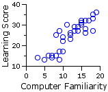
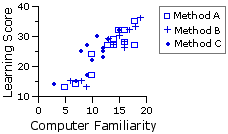
The reason for this shortfall is of course the degree of variability within the groups, which is quite large in comparison with the mean differences that appear between the groups. Well aware of the broad range of pre-existing individual differences that are likely to be found in situations of this sort, our curriculum researcher took the precaution of measuring her subjects beforehand with respect to their pre-existing levels of basic computer familiarity. The rationale is fairly obvious: the more familiar a subject is with basic computer procedures, the more of a head start he or she will have in learning the elements of computer programming; remove the effects of this covariate, and you thereby remove a substantial portion of the extraneous individual differences. Our researcher was also well aware that her three groups, drawn from three different schools, might be starting out with substantially different levels of basic computer familiarity, in consequence of the average socio-economic differences that she knows to exist among the schools. The groups instructed by Methods A and B both reside in fairly affluent neighborhoods, while the group instructed by Method C comes from a less privileged part of town.

The following table shows the measures on both variables laid out in a form suitable for an analysis of covariance, with

	X =	the prior measure of basic computer familiarity [The covariate whose effects the investigator wishes to remove from the analysis.]
and
	Y =	the measure of how well the subject has learned the elementary programming material [The dependent variable in which the investigator is chiefly interested.]

---

		Method A				Method B				Method C
	Sub- ject	Xa	Ya		Sub- ject	Xb	Yb		Sub- ject	Xc	Yc
	a1  a2  a3  a4  a5  a6  a7  a8  a9  a10  a11  a12	14  10  7  18  14  16  13  15  5  18  16  10	29 24 14 27 27 28 27 32 13 35 32 17		b1  b2  b3  b4  b5  b6  b7  b8  b9  b10  b11  b12	6  16  9  19  13  14  15  18  17  8  15  16	15 28 13 36 29 27 31 33 32 15 30 26		c1  c2  c3  c4  c5  c6  c7  c8  c9  c10  c11  c12	15  9  7  12  12  9  12  3  13  10  11  8	32 27 15 23 26 17 25 14 29 22 30 25
Means		13.0	25.4			13.8	26.3			10.1	23.8

As you can see from the means in the X columns, the investigator was right in her expectations concerning different group levels of basic computer familiarity: 13.0 and 13.8 for groups A and B, versus 10.1 for group C. So once again we encounter the what-if question: What would have happened if the three groups had all started out on the same footing?

---

The computational format for the one-way ANCOVA is the same here as for Example 1. The only structural difference is that now the number of groups is k=3.

---

1. Calculations for the Dependent Variable Y

Values of Y along with the several summary statistics required for the calculation of SS_T(Y), SS_wg(Y), and SS_bg(Y):

	Ya	Yb	Yc
	29 24 14 27 27 28 27 32 13 35 32 17	15 28 13 36 29 27 31 33 32 15 30 26	32 27 15 23 26 17 25 14 29 22 30 25	for total array of data
N	12	12	12	36		SST(Y) = 1626.3  SSwg(Y) = 1587.5  SSbg(Y) = 38.9
.Yi	305	315	285	905
.Yi2	8315	8919	7143	24377
SS	562.9	650.3	374.3
Mean	25.4	26.3	23.8	25.1

---

2. Calculations for the Covariate X

Values of X along with the several summary statistics required for the calculation of SS_T(X) and SS_wg(X).

	Xa	Xb	Xc
	14   10   7   18   14   16   13   15   5   18   16   10	6   16   9   19   13   14   15   18   17   8   15   16	15   9   7   12   12   9   12   3   13   10   11   8	for total array of data
N	12	12	12	36		SST(X) = 581.6  SSwg(X) = 488.6
.Xi	156	166	121	443
.Xi2	2220	2482	1331	6033
SS	192.0	185.7	110.9
Mean	13.0	13.8	10.1	12.3

---

3. Calculations for the Covariance of X and Y

Cross-products of X_i and Y_i for each subject in each of the three groups, along with other summary data required for the calculation of SC_T and SC_wg:

A	B	C
XaYa	XbYb	XcYc
(14)(29) = 406 (10)(24) = 240 (7)(14) =98 (18)(27) = 486 (14)(27) = 378 (16)(28) = 448 (13)(27) = 351 (15)(32) = 480 (5)(13) =65 (18)(35) = 630 (16)(32) = 512 (10)(17) = 170	(6)(15) =90 (16)(28) = 448 (9)(13) = 117 (19)(36) = 684 (13)(29) = 377 (14)(27) = 378 (15)(31) = 465 (18)(33) = 594 (17)(32) = 544 (8)(15) = 120 (15)(30) = 450 (16)(26) = 416	(15)(32) = 480 (9)(27) = 243 (7)(15) = 105 (12)(23) = 276 (12)(26) = 312 (9)(17) = 153 (12)(25) = 300 (3)(14) =42 (13)(29) = 377 (10)(22) = 220 (11)(30) = 330 (8)(25) = 200	for total array of data
.∑(XaiYai) =4264	.∑(XbiYbi) =4683	.∑(XciYci) =3038	.∑(XTiYTi) =11985
o∑Xai=156 o∑Yai=305	o∑Xbi=166 o∑Ybi=315	o∑Xci=121 o∑Yci=285	o∑XTi=443 o∑YTi=905

---

Calculation of SC for the total array of data:

SCT

= ∑(XTiYTi) —

(∑XTi)(∑YTi) NT

SCT

= 11985 —

(443)(905) 36

= 848.5

---

Calculation of SC_wg:

The components for each group ("g") are calculated as:

SCwg(g)

= ∑(XgiYgi) —

(∑Xgi)(∑Ygi) Ng

Thus:

SCwg(a)

= 4264 —

(156)(305) 12

= 299.0

SCwg(b)

= 4683 —

(166)(315) 12

= 325.5

SCwg(c)

= 3036 —

(121)(285) 12

= 164.3

	SCwg	= SCwg(a) + SCwg(b) + SCwg(c)
		= 299.0 + 325.5 + 164.3 = 788.8

---

4. The Final Set of Calculations

Here again is a summary of the values of SS and SC obtained so far. Recall that Y is the variable in which we are chiefly interested, and X is the covariate whose effects we are seeking to remove.

	X		Y		Covariance
	SST(X) = 581.6 SSwg(X) = 488.6		SST(Y) = 1626.3 SSwg(Y) = 1587.4 SSbg(Y) = 38.9		SCT = 848.5 SCwg = 788.8
	For handy reference, click here to place a version of this table into the frame on the left.]

---

4a. Adjustment of SS_T(Y)

As indicated in connection with Example 1, the overall correlation between X and Y (all three groups combined) can be calculated as

	rT	=	SCT sqrt[SST(X) x SST(Y)]
		=	848.5 sqrt[581.6 x 1626.31]
		=	+.872

The proportion of the total variability of Y attributable to its covariance with X is accordingly

(rT)2 = (+.872)2 = .760

As previously noted, the removal of this portion is best accomplished (minimizing the risk of rounding errors) through the computational formula

	[adj]SST(Y)	= SST(Y)—	(SCT)2 SST(X)
		= 1626.3 —	(848.5)2 581.6
		= 388.4

---

4b. Adjustment of SS_wg(Y)

Similarly, the aggregate correlation between X and Y within the three groups can be calculated as

	rwg	=	SCwg sqrt[SSwg(X) x SSwg(Y)]
		=	788.8 sqrt[488.6 x 1587.4]
		=	+.896

So the proportion of the within-groups variability of Y attributable to covariance with X is

(rwg)2 = (+.896)2 = .803

Here again, the removal of this portion is best accomplished through the computational formula

	[adj]SSwg(Y)	= SSwg(Y)—	(SCwg)2 SSwg(X)
		= 1587.4 —	(788.8)2 488.6
		= 314.0

---

4c. Adjustment of SS_bg(Y)

The adjusted value of SS_bg(Y) can then again be obtained through simple subtraction as

	[adj]SSbg(Y)	=	[adj]SST(Y) — [adj]SSwg(Y)
		=	388.4 — 314.0 = 74.4

---

4d. Adjustment of the Means of Y for Groups A, B, and B

The average relationship between X and Y within the groups is given by the slope of the regression line for the within-groups correlation, which is

	bwg	=	SCwg SSwg(X)
		=	788.8 488.6	= +1.61

The logic here is the same as with Example 1. The three groups started out with different average levels of basic computer familiarity. Suppose they had instead all started out with the same level: namely, 12.3, which is the mean of X for all three groups combined. In this case, group A would have been starting out with a mean familiarity level 0.7 units lower than it actually started with; group B would have been starting out 1.5 units lower; and group C would have been starting out 2.2 units higher. Given the observed dependance of Y on X, the respective means of Y for the three groups would presumably therefore have been on the order of

	[adj]MYa	= MYa — bwg(MXa—MXT)
		= 25.4 — 1.61(13.0—12.3)
		= 24.3

	[adj]MYb	= MYb — bwg(MXb—MXT)
		= 26.3 — 1.61(13.8—12.3)
		= 23.9

	[adj]MYc	= MYc — bwg(MXc—MXT)
		= 23.8 — 1.61(10.1—12.3)
		= 27.3

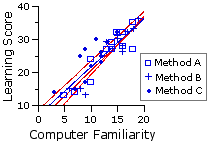
As illustrated in the adjacent graph, the adjusted group means paint quite a different picture. When the different pre-existing levels of basic computer familiarity are taken into account, Method C appears to have a substantial edge over both of the other instructional methods.

---

4e. Analysis of Covariance Using Adjusted Values of SS

The simple computational format for this step is the same as for Example 1. All we need do here is lay out its results in the form of an ANCOVA summary table:

	Source	SS	df	MS	F	P
	adjusted means   [between-groups effect]	74.4	2	37.2	3.8	<.05
	adjusted error   [within-groups]	314.0	32	9.8
	adjusted total	388.4	34

[Recall that  dfbg(Y)=k—1  and  [adj]dfwg(Y)=NT—k—1]

As you can see from the adjacent portion of Appendix D, the calculated value of F=3.8 is significant beyond the .05 level for df=2,32. Once again, let me note that a significant ANCOVA result of this sort does not refer to the observed means of the samples, but to the adjusted means. It is the same chain of if/then constructions laid out in Example 1:

• If the correlation between X and Y within the general population is approximately the same as we have observed within the samples; and_T
  
• If we remove from Y the covariance that it has with X, so as to remove from the analysis the pre-existing individual differences that are measured by the covariate X; and_T
  
• If we adjust the group means of Y in accordance with the observed correlation between X and Y;_T
  
• Then we can conclude that the three adjusted means significantly differ in the degree indicated, namely, P<.05.

In the present case it is fairly obvious to the naked eye that the bulk of this effect is contributed by Method C, which our curriculum researcher could reasonably conclude to be more effective than either of the other two methods, given this particular population of subjects.

---

¶Test for Homogeneity of Regression

As mentioned toward the end of Part 2, the analysis of covariance assumes that the slopes of the regression lines for each of the groups considered separately do not significantly differ from the slope of the overall within-groups regression, which for the present example is b_wg=+1.61. If they do significantly differ, then the analysis of covariance is invalid and any positive conclusion drawn from it is potentially false and misleading.

In the adjacent graph you can see that the three separate group regression lines, in red, do appear to be in close parallel with the blue line for the overall within-groups regression. However, here as elsewhere in the domain of statistical inference, a merely intuitive impression of this sort is not sufficient. For the naked eye is simply not capable of making the fine-grained distinctions that need to be made with complex sets of numerical data.

The procedure for rigorously determining whether this "homogeneity of regression" assumption is satisfied involves yet another variation on the theme of analysis of variance. As in all versions of ANOVA, the end result is an F-ratio of the general form

F =

MSeffect MSerror

=

SSeffect /dfeffect SSerror /dferror

---

Numerator SS

In the present version, the sum of squared deviates (SS_effect) in the numerator of the ratio is a measure of the aggregate degree to which the separate regression-line slopes of the several groups differ from the slope (b_wg) of the line for the overall within-groups regression. We will henceforth designate this quantity as SS_b-reg ("b-reg" = "between regressions"). As the rationale for this SS_b-reg measure is a bit more intricate than we need to get into just now, I will present it simply as a matter of computational mechanics.

1. For each group ("g"), calculate
   

   (SCg)2 SSXg

   
   

   Note thatSCg/SSXg would give you the slope for group g.

   
   
2. Sum up the results of step 1 and subtract from that sum the quantity
   

   (SCwg)2 SSwg(X)

   
   

   Note thatSCwg/SSwg(X) = bwg the slope for the overall within-groups regression.

   
   Hence:
   

   SSb-reg =

   (SCg)2 SSXg

   —

   (SCwg)2 SSwg(X)

   
   which for the present example, using previously calculated values, comes out to

   SSb-reg

   =

   (SCa)2 SSXa

   +

   (SCb)2 SSXb

   +

   (SCc)2 SSXc

   —

   (SCwg)2 SSwg(X)

   SSb-reg

   =

   (299.0)2 192.0

   +

   (325.5)2 185.7

   +

   (164.3)2 110.9

   —

   (788.8)2 488.6

   SSb-reg

   =

   6.1

---

Denominator SS

The sum of squared deviates (SS_error) in the denominator of the F-ratio is reached much more easily. We will designate this quantity as SS_Y(remainder), because it is simply what is left over from [adj]SS_wg(Y), the "adjusted error" of the original ANCOVA, after SS_b-reg has been removed from it. Thus

	SSY(remainder)	= [adj]SSwg(Y) — SSb-reg
		= 314.0 — 6.1 = 307.9
		= 307.9

---

df

The apportionment of degrees of freedom follows the same pattern. The value of [adj]SS_wg(Y) that appears in the original ANCOVA starts out with degrees of freedom equal to

	[adj]dfwg(Y)	= NT — k — 1
		= 36 — 3 — 1
		= 32

When you remove SS_b-reg from [adj]SS_wg(Y), you are also removing the number of degrees of freedom that go along with it, which is

	dfb-reg	= k — 1
		= 3 — 1
		= 2

So the degrees of freedom for SS_Y(remainder) is

	dfY(remainder)	= [adj]dfwg(Y) — dfb-reg
		= (NT—k —1)—(k —1)
		= 32 — 2 = 30

As a computational expedient, you can also
calculate [adj]df_wg(Y) as N_T—2k.

---

With these components at hand we can then calculate the F-ratio for homogeneity of regression as

	F	=	MSb-reg MSY(remainder)	=	SSb-reg /dfb-reg SSY(remainder) /dfY(remainder)
		=	6.1/2 307.9/30
		=	0.30	[with df = 2,30]

df denomi- nator	df numerator
	1	2	3
30	4.17 7.56	3.32 5.39	2.92 4.51

Here on the right is the relevant portion of Appendix D, though with such a tiny F-ratio one need hardly bother to consult it. As we noted in Chapter 13, any value of F equal to or smaller than 1.0 will be non-significant. At any rate, the slopes of the three separate group regression lines do not significantly differ from b_wg=+1.61. Hence the assumption of homogeneity of regression is satisfied.

---

In Chapter 18 we will extend the analysis of covariance to the case where there are two independent variables, on analogy with the two-way analysis of variance for independent samples examined in Chapter 16.